Under Construction
This page is currently being rebuilt. Please check back soon!
Back to PortfolioProject 6: Pre-canned Projects
By Danial Toktarbayev and Mustafa Mirza
For our final project we did three projects: Light Field Camera, High Dynamic Range Imaging, and Gradient Fusion Domain
Task 1 - Depth Refocusing
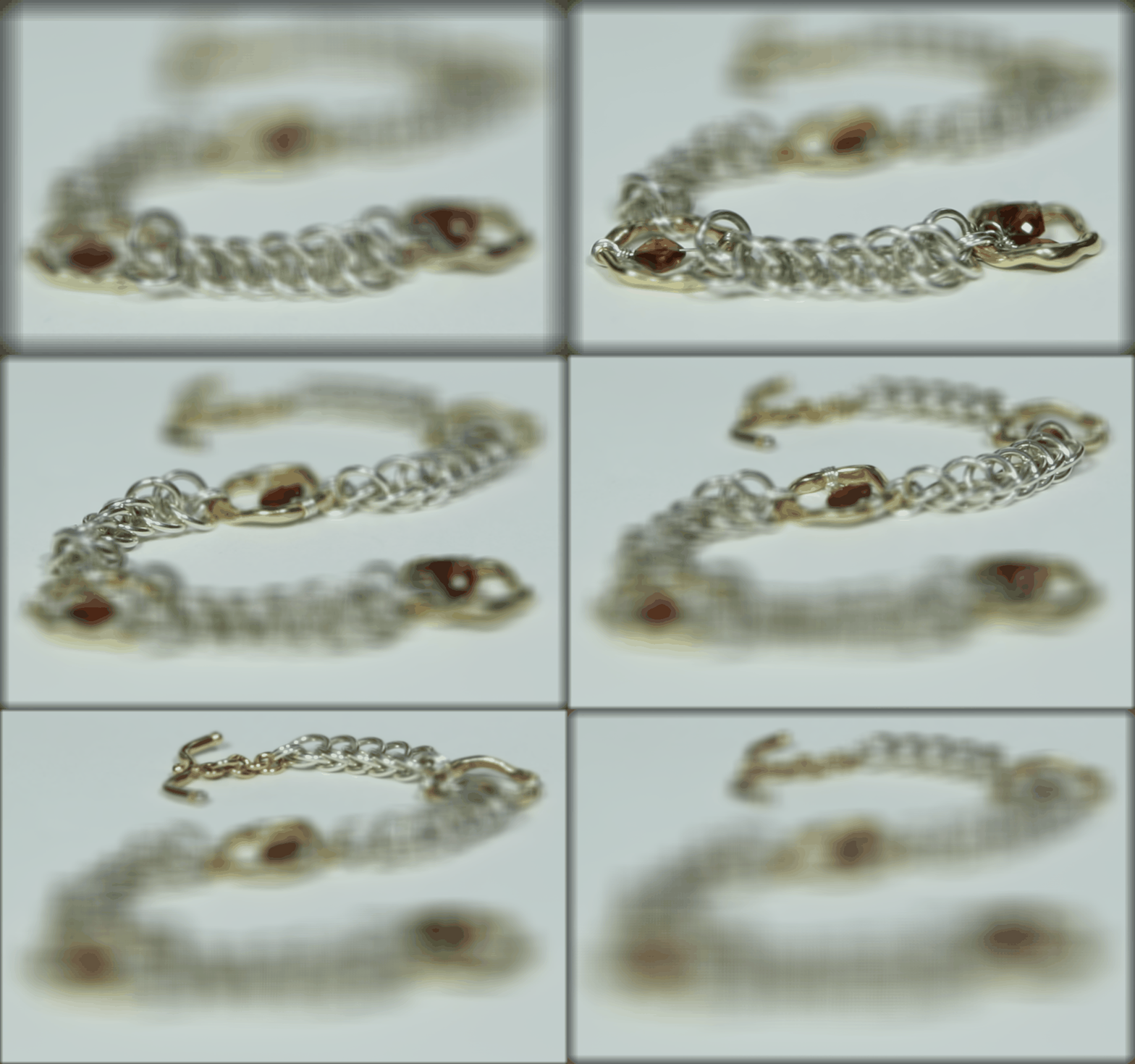
In this task, we implemented digital refocusing using light field data captured from a grid of camera positions. We processed multiple images from the Stanford Light Field Archive by applying perspective shifts based on camera positions and combining them to achieve selective focus at different depths. The key insight was that objects at different depths exhibit varying parallax across the image grid - distant objects show minimal position changes while nearby objects show significant shifts. By calculating appropriate perspective transformations and combining the shifted images, we could control which depth appears sharp in the final image. Our implementation used the concept that averaging aligned images after applying depth-dependent shifts allows us to synthetically adjust the focal plane after capture.
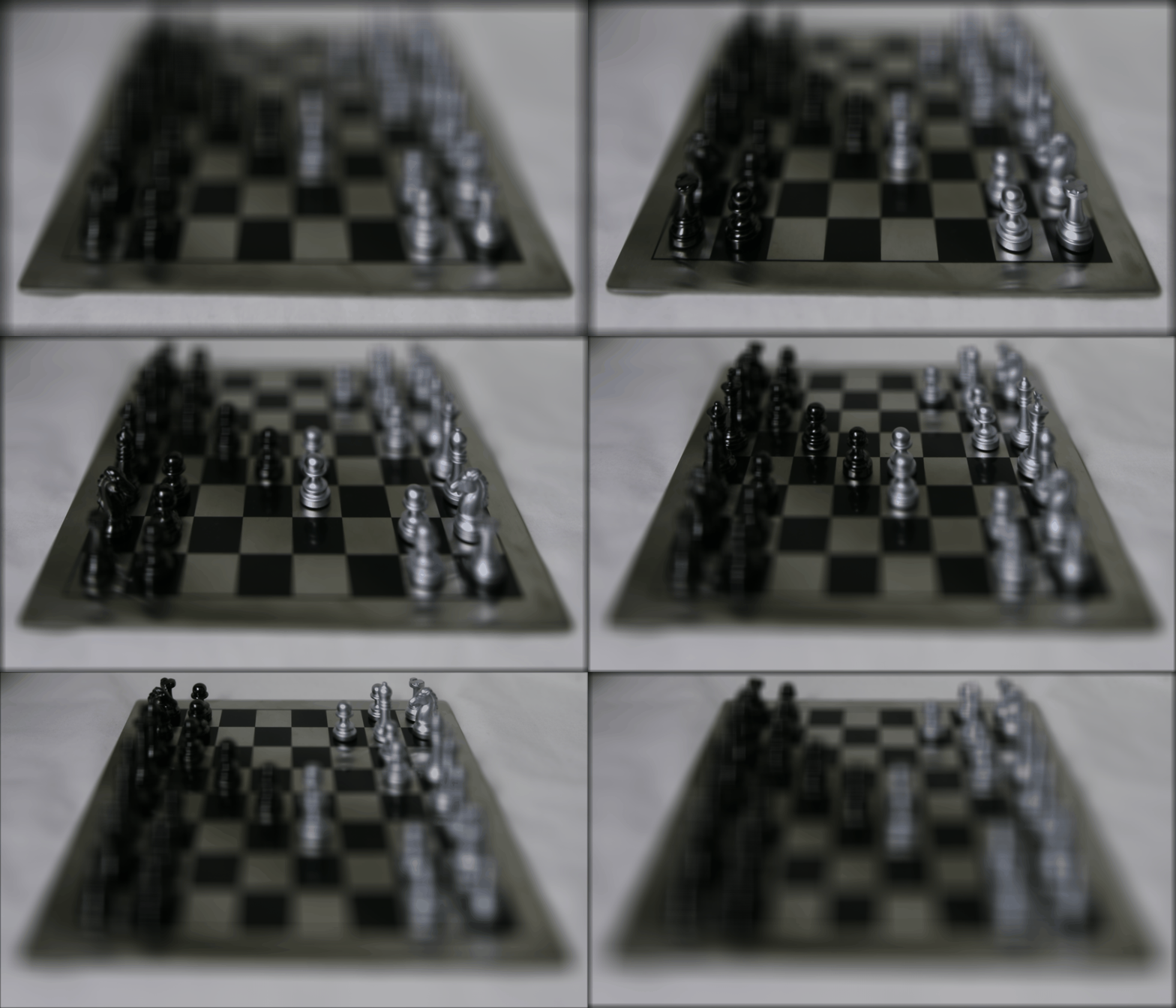
We did the same thing with other pics too, and here's what we got:
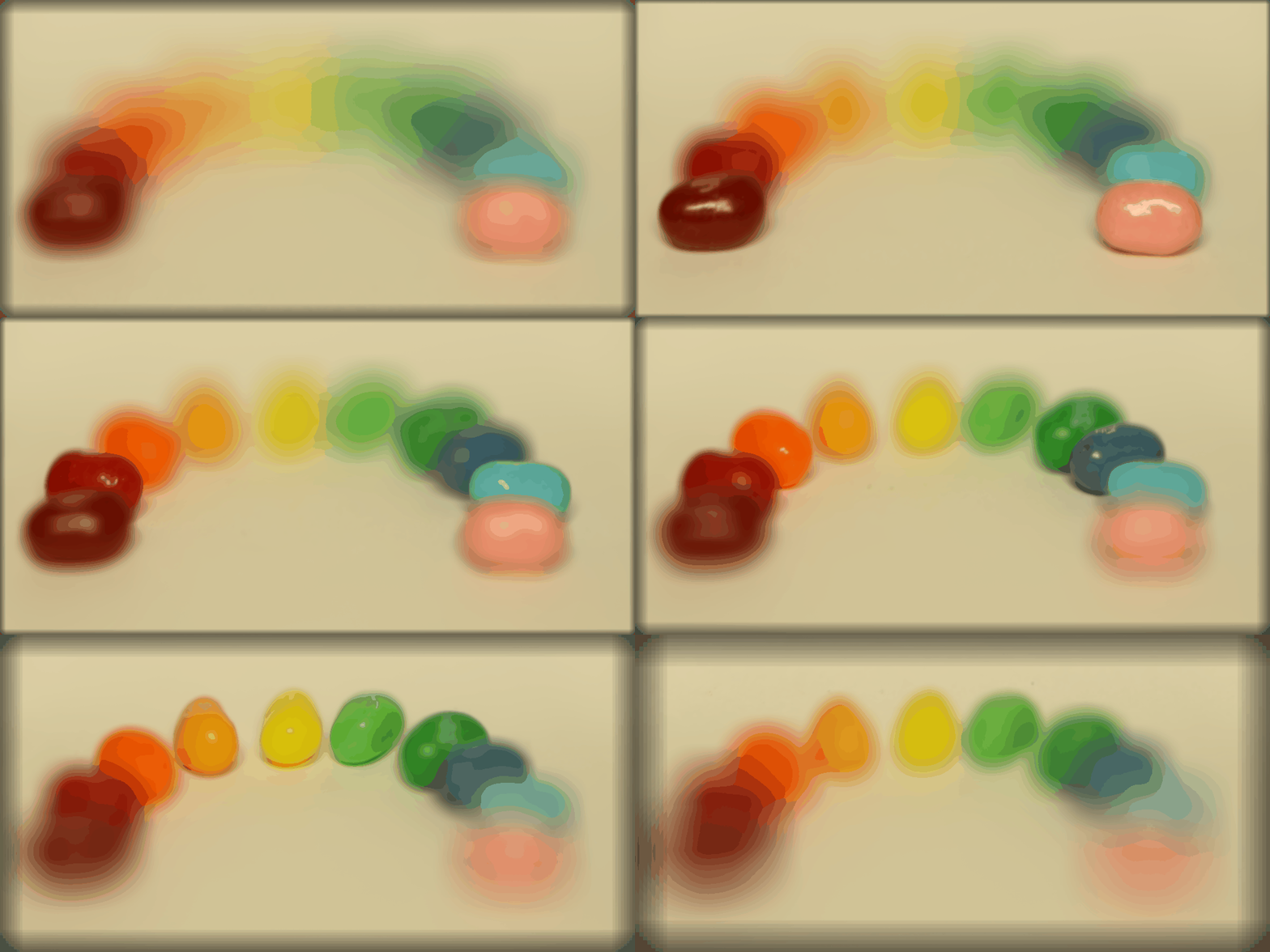
Task 2 - Apertures
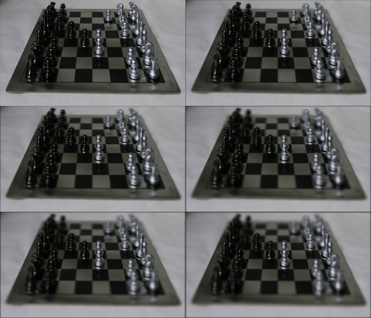
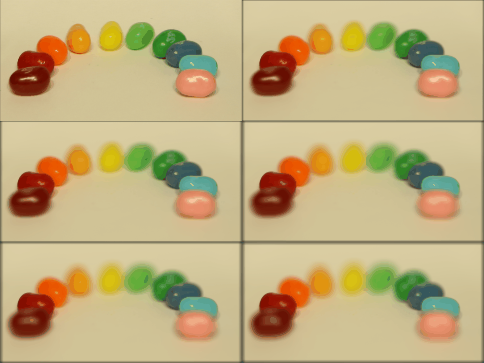
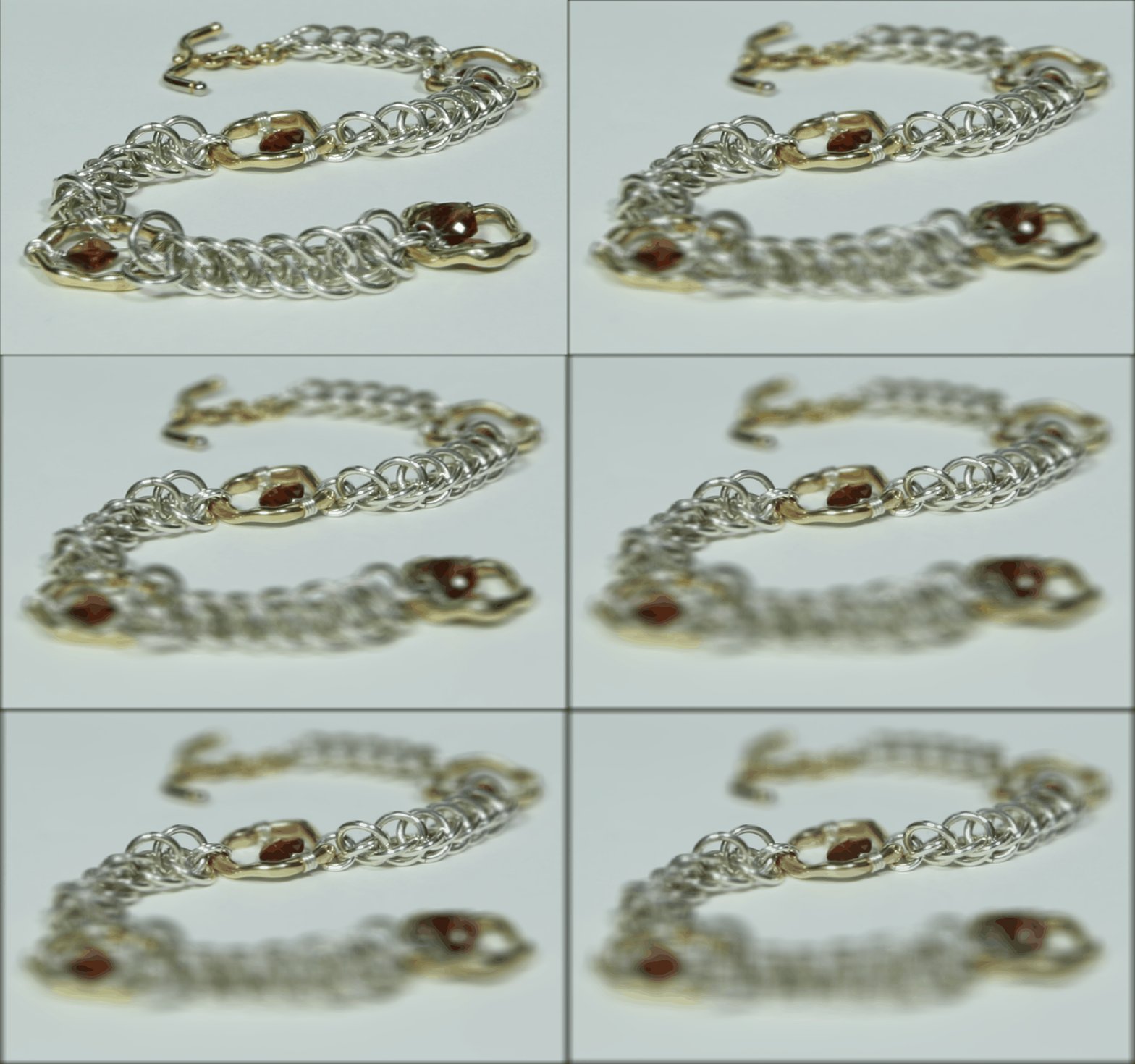
For the aperture adjustment task, we simulated different lens aperture sizes by selectively combining subsets of the light field images. We implemented this by filtering perspective shifts based on their magnitudes - using more shifts corresponds to a larger synthetic aperture while fewer shifts creates a smaller effective aperture. In our code, we used numpy arrays to calculate maximum allowed displacement and implemented filtering using a simple distance-based threshold that determined which camera positions to include. For each aperture value in our test range (0.1 to 1.0), we created filtered subsets of the perspective shifts and their corresponding images, then combined them to generate the final synthetic photographs. This demonstrated how light field capture enables post-capture aperture control, allowing us to trade off depth of field versus light gathering after the fact. The implementation helped us understand how simple geometric constraints and image averaging can simulate complex optical effects.
Summary
Through this project, we learned how capturing multiple regular 2D photographs from different viewpoints arranged in a grid can enable powerful computational photography effects. By processing these multi-view images using perspective shifts and selective averaging, we could simulate effects like refocusing at different depths and adjusting the apparent aperture size after capture. The project demonstrated that even without specialized light field camera hardware, we can achieve interesting computational photography capabilities by clever processing of multiple standard photographs taken from different positions. This helped us understand both the power and limitations of multi-view image processing for creating synthetic photographic effects.
Bells & Whistles: Interactive Refocusing
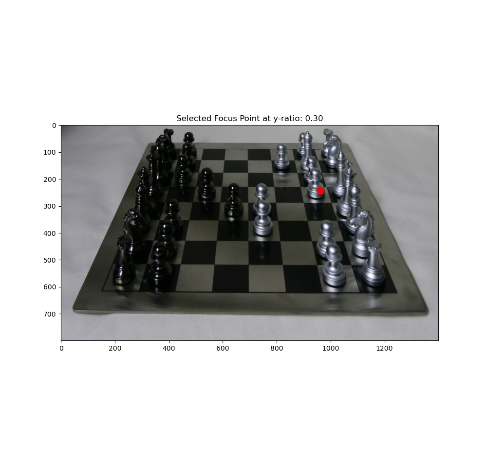
Interactive point selection
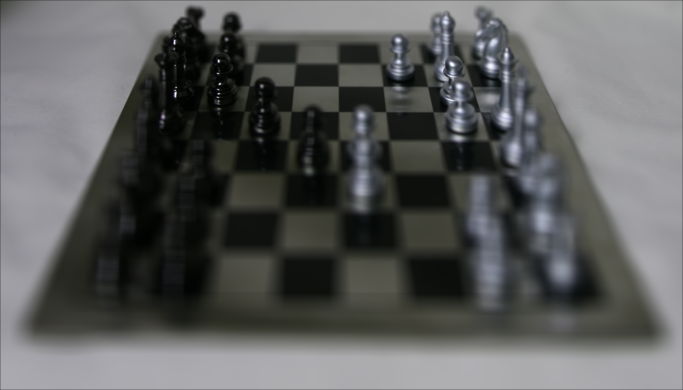
Refocused result
Radiance Map Construction
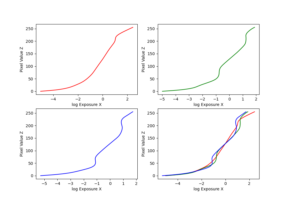
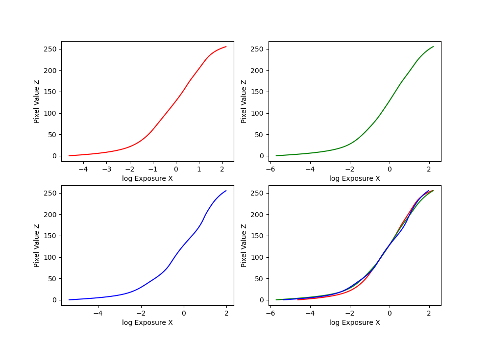
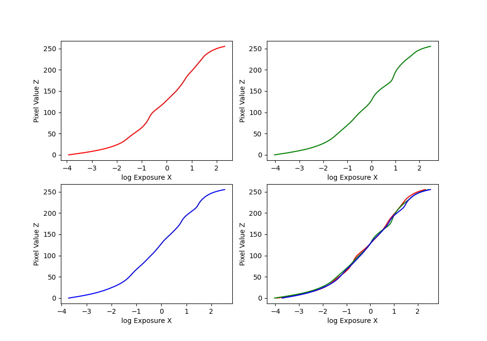
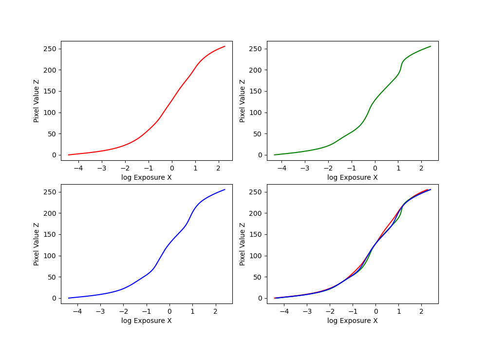
We have several images of the same place with different exposures. First, we implemented a function solve_g given to us in starter code. This is basically implementing least squares algorithm to estimate g and unknown ln(E_i) for each pixel, based on on the i-th pixel in image j. Here's the formula: \[ \mathcal{O} = \sum_{i=1}^{N} \sum_{j=1}^{P} \left[ g(Z_{ij}) - \ln E_i - \ln \Delta t_j \right]^2 + \lambda \sum_{z=Z_{\text{min}}+1}^{Z_{\text{max}}-1} \left[ g''(z) \right]^2 \]
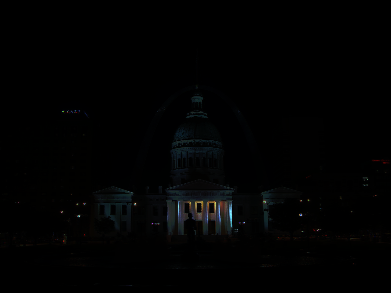
Here's a few graphs that we got for different images (arch, chapel, and window):
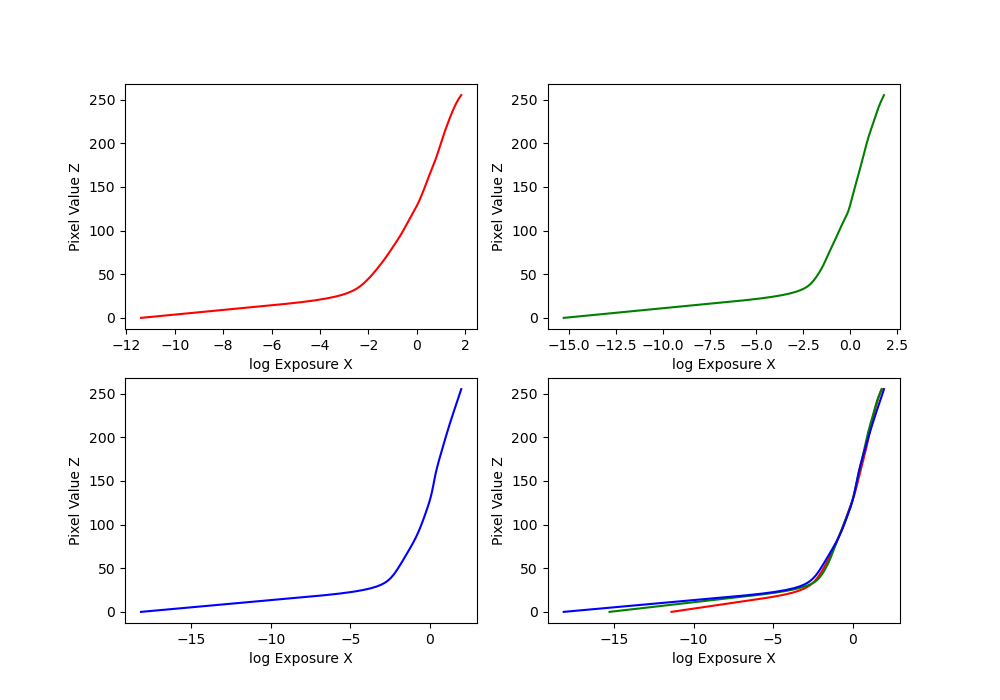
Bonsai and garage:
Bonsai log exposure
Garage log exposure
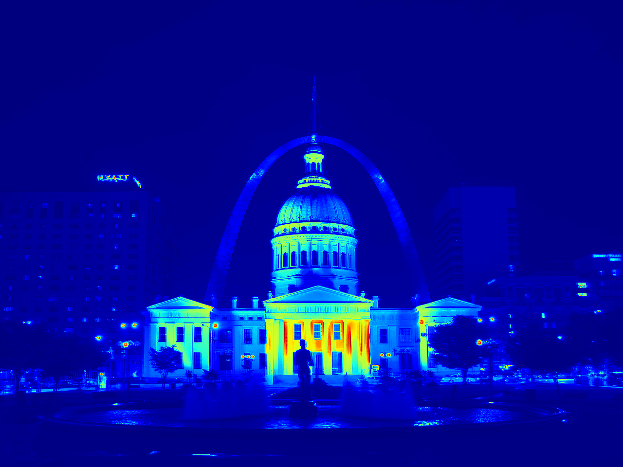
Our Radiance Maps
Arch, chapel, and window:
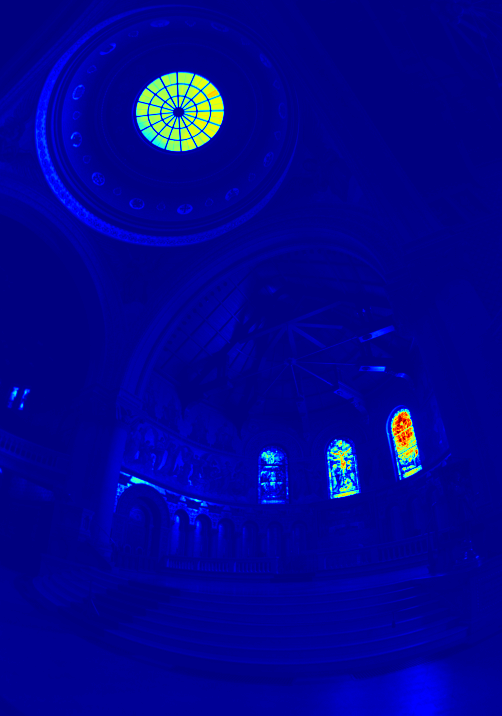
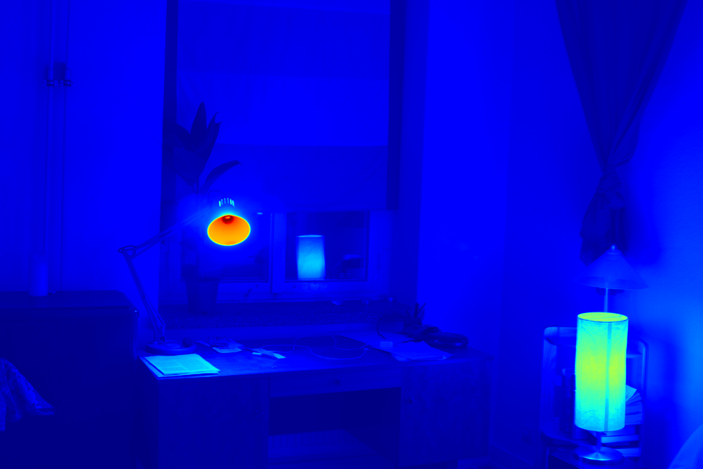
Bonsai and garage:
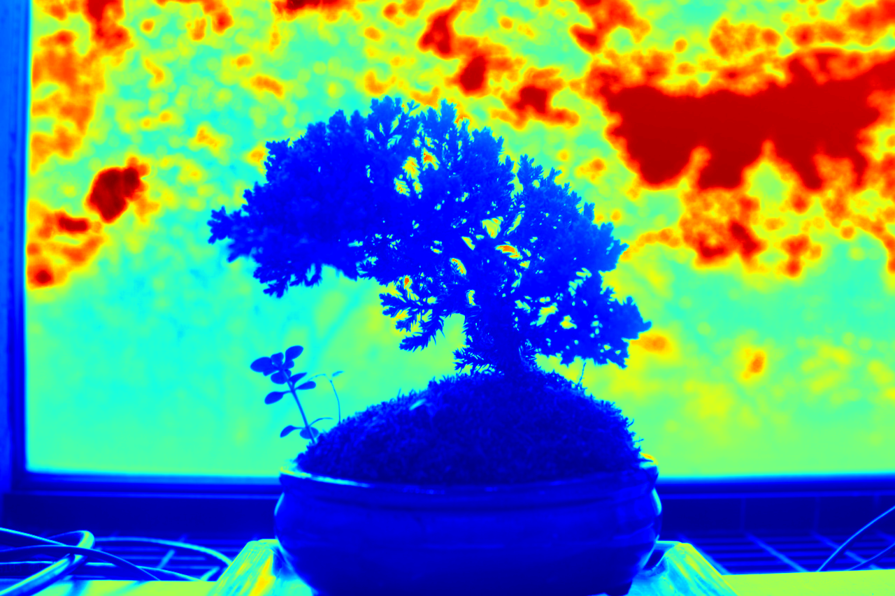
Bonsai radiance map
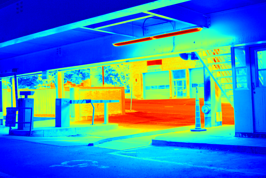
Garage radiance map
Tone Mapping
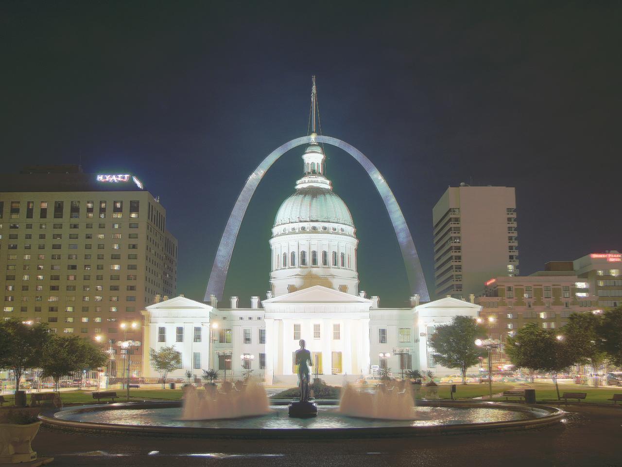
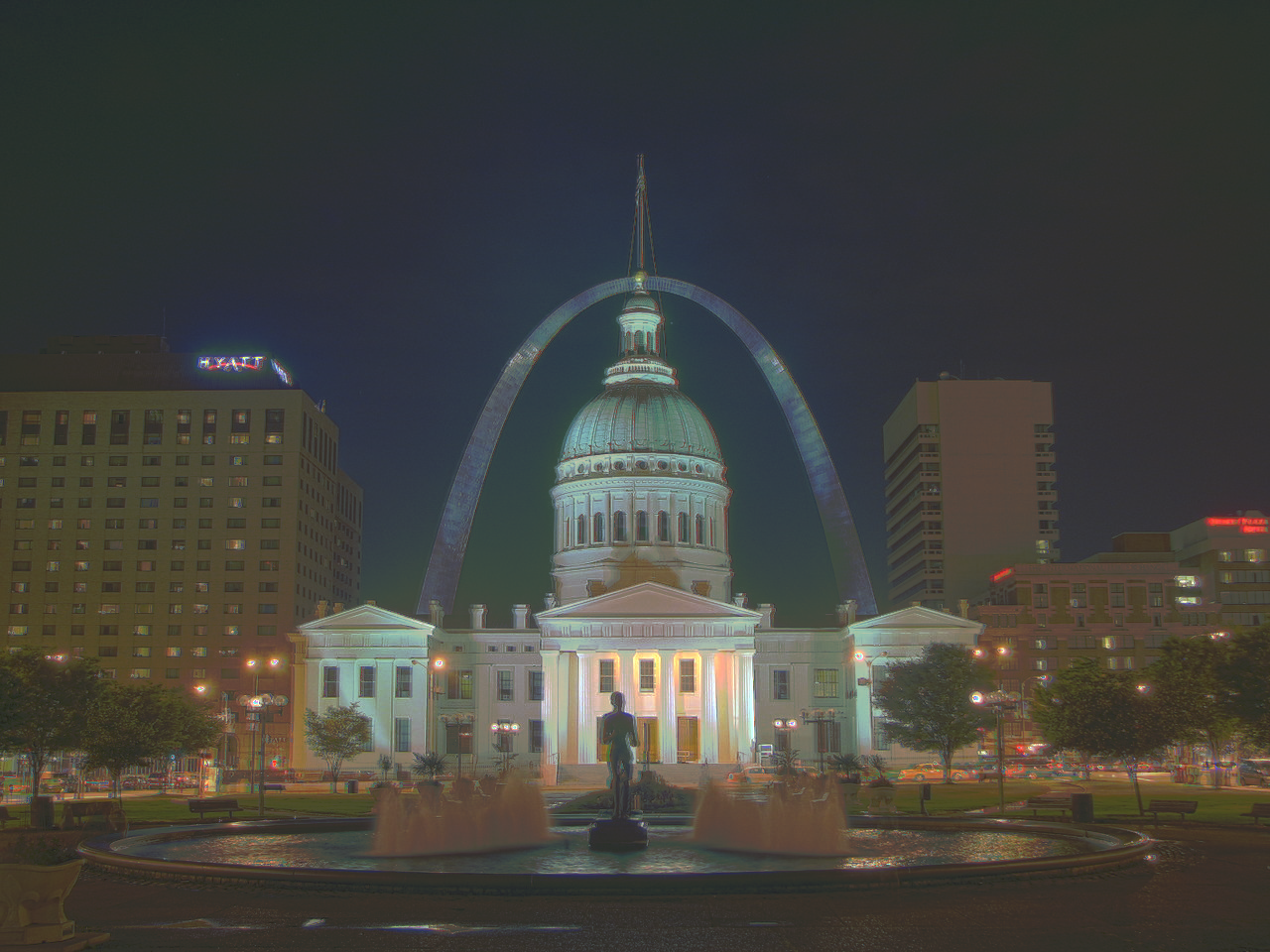
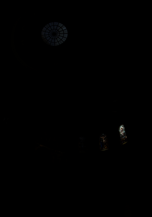
Now we want to clearly show the image, for which we compute global intensity (averaging) and scale colors by it.
Arch global scaling
Arch global simple
Durand
Chapel global scaling
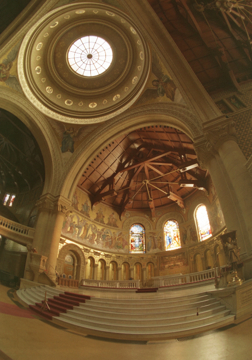
Global simple
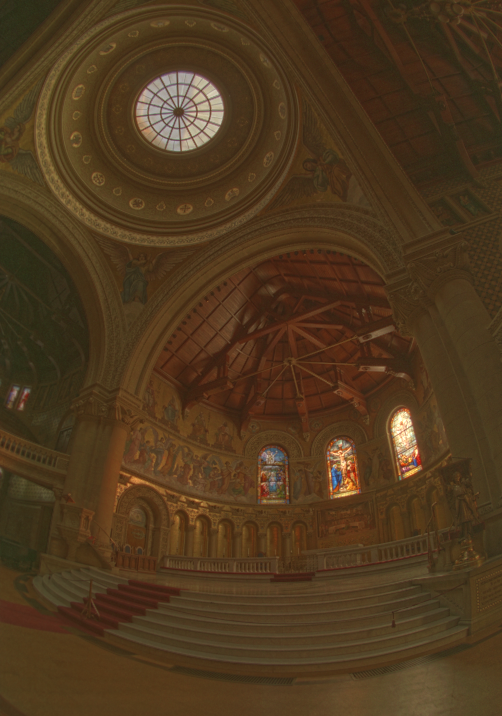
Durand
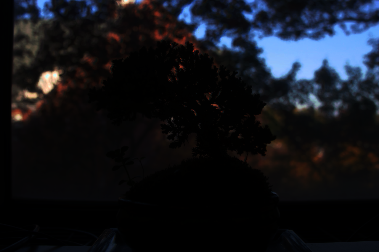
Bonsai global scaling
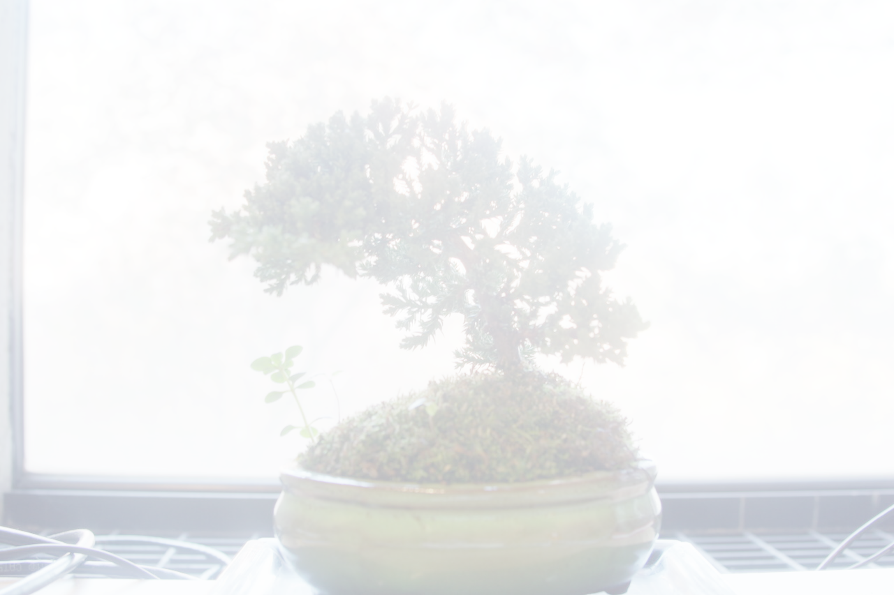
Global simple
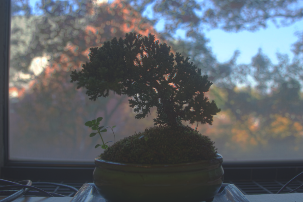
Durand
Bells & Whistles: Local Tone Mapping Algorithm
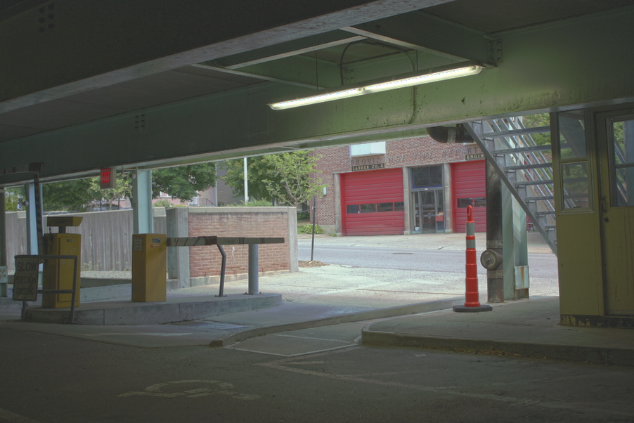
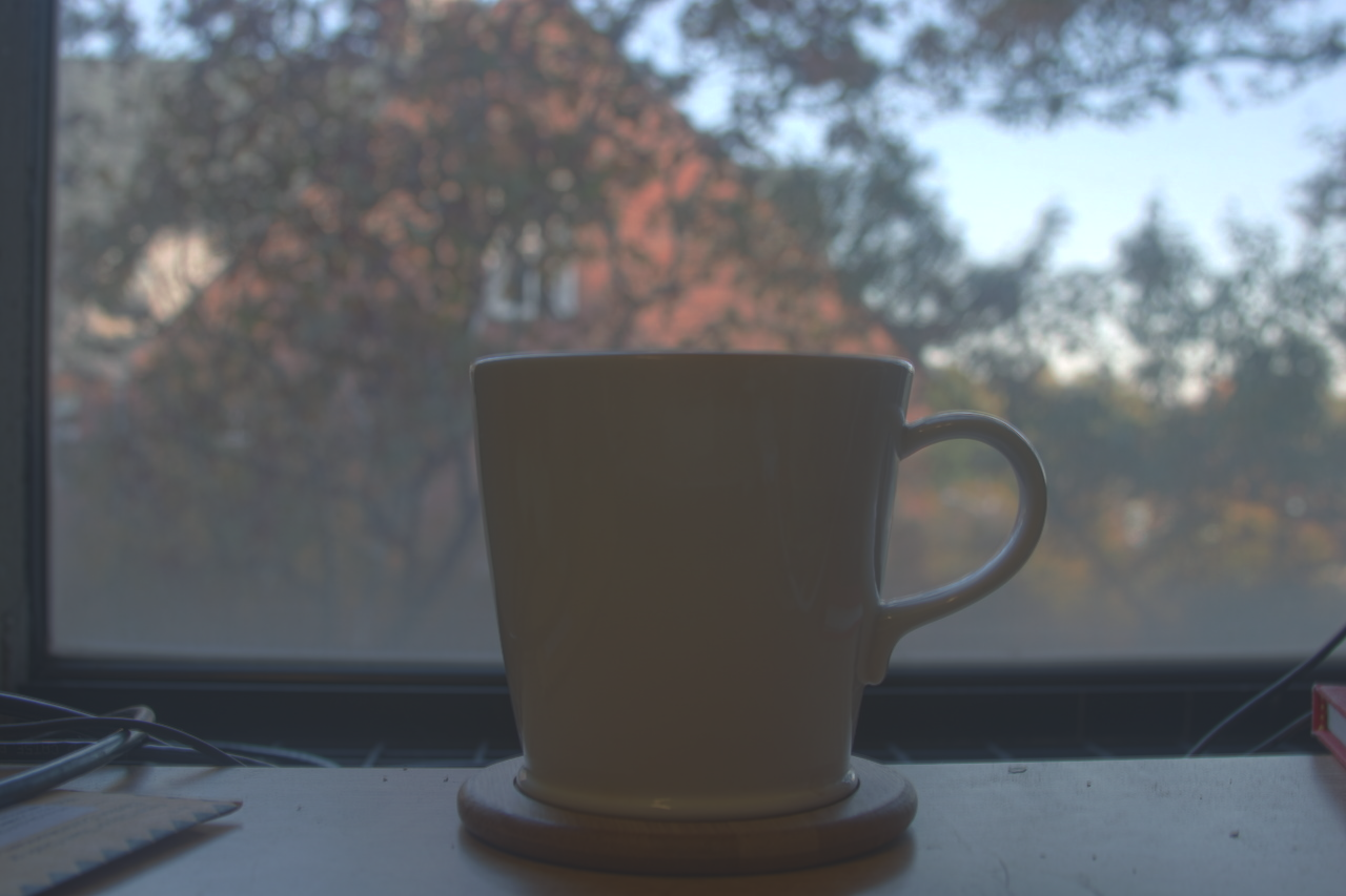
Simplified local tone mapping algorithm using Gaussian pyramids for local contrast adjustment. Results below:
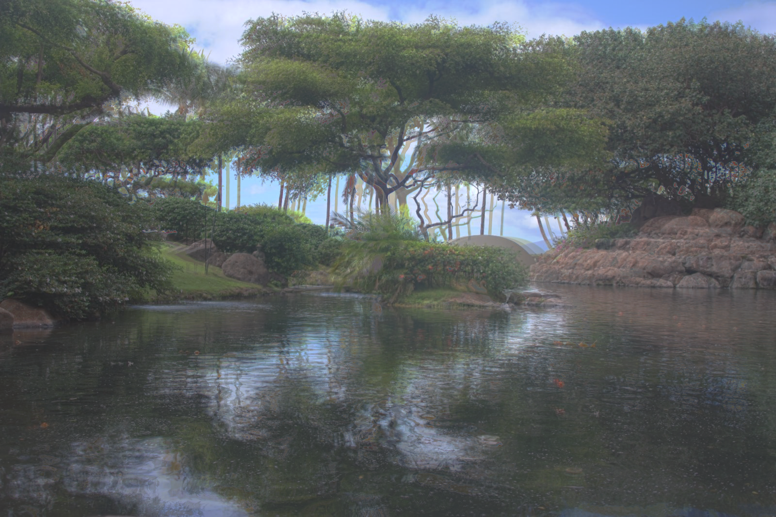


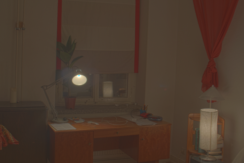

Chapel with local tone mapping
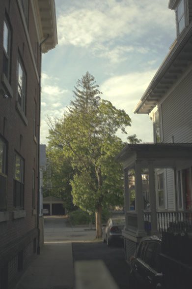
House with local tone mapping
Summary
This project taught us to create high dynamic range images by combining multiple exposures. We were introduced to the Debevec and Malik 1997 method. Additionally learned adding global and local tone to make the radiance map displayable. Even though local tone does not look as good as global tone, it taught us a different technique.
Toy Problem
So in this part we're trying to recreate the image by computing the x and y gradients from a source image plus one pixel intensity. The formula looks like this: minimize ( v(x+1,y)-v(x,y) - (s(x+1,y)-s(x,y)) )^2, minimize ( v(x,y+1)-v(x,y) - (s(x,y+1)-s(x,y)) )^2, and minimize (v(1,1)-s(1,1))^2 where s in intensity of source image at x, y, and v is the value of the image at x, y. Results are below:
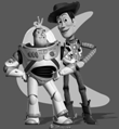
Original image
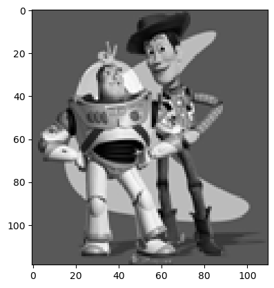
Recreated image
Poisson Blending
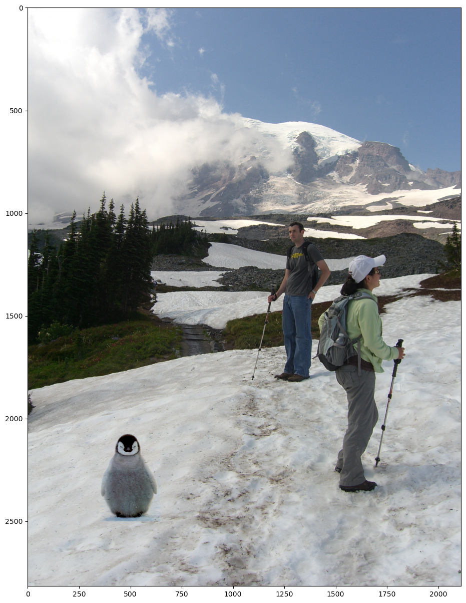
Used the function below to minimize the intensity of gradients between the source and background images within the masked area. Poisson blessing showed better results than Laplacian pyramid, even though it looks like the background of source image did not fully disappear. $$ \mathbf{v} = \arg\min_{\mathbf{v}} \sum_{i \in S, j \in N_i \cap S} \left( (v_i - v_j) - (s_i - s_j) \right)^2 + \sum_{i \in S, j \in N_i \cap \neg S} \left( (v_i - t_j) - (s_i - s_j) \right)^2 $$
Example 1: Penguin Chick
Background and source images:
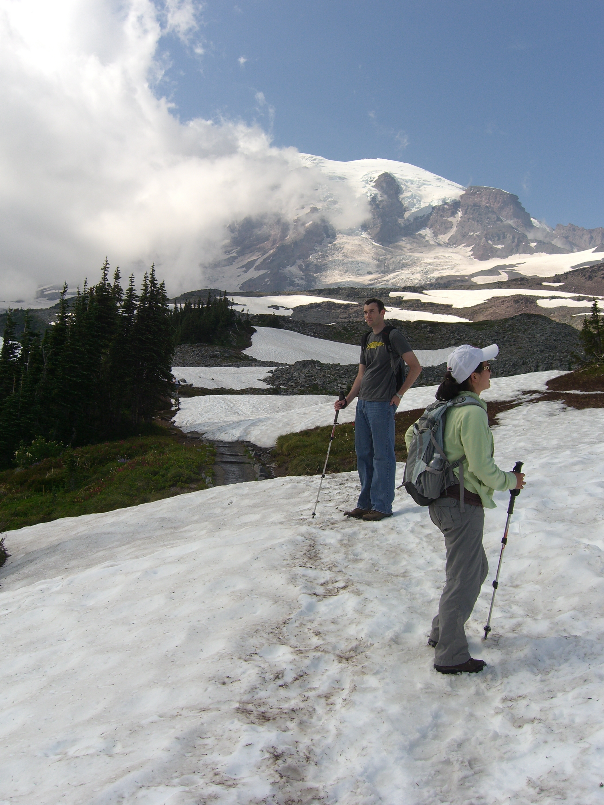
Background image
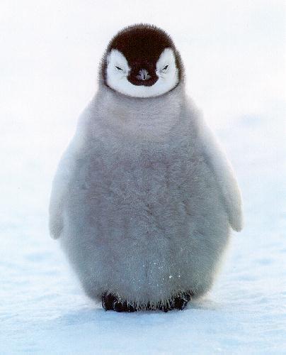
Source image

Initial preparation
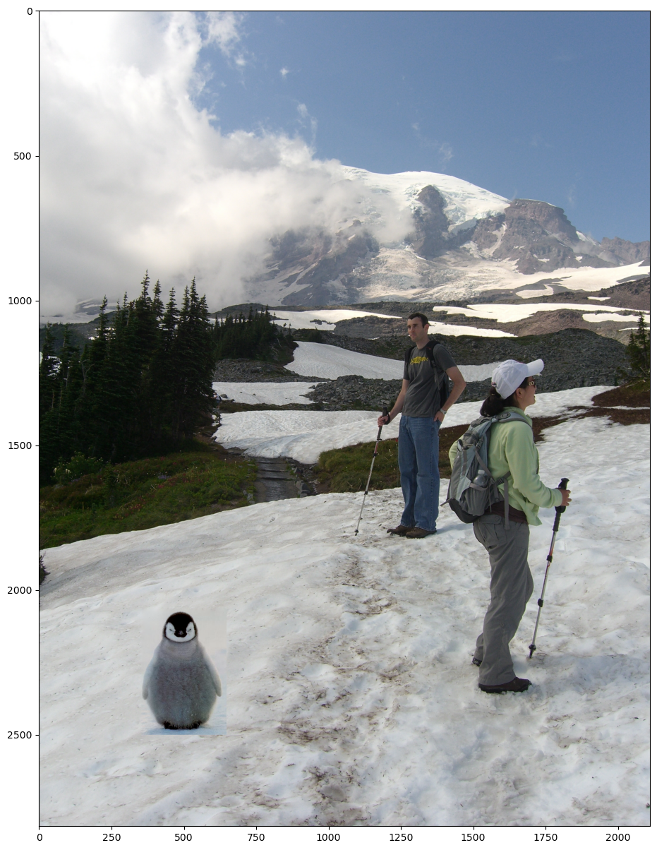
Poisson blending result
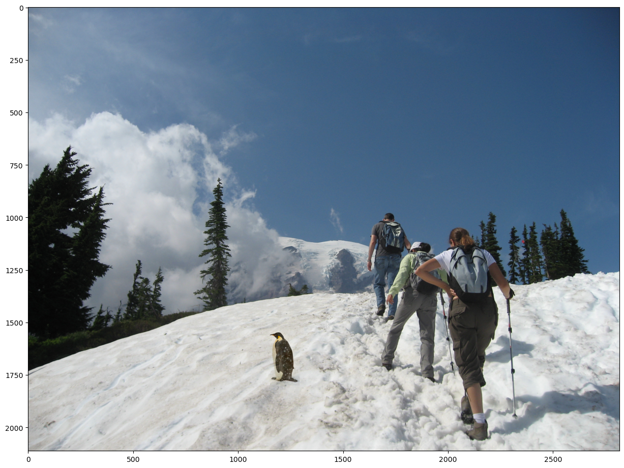
Example 2: Penguin
Background and source images:
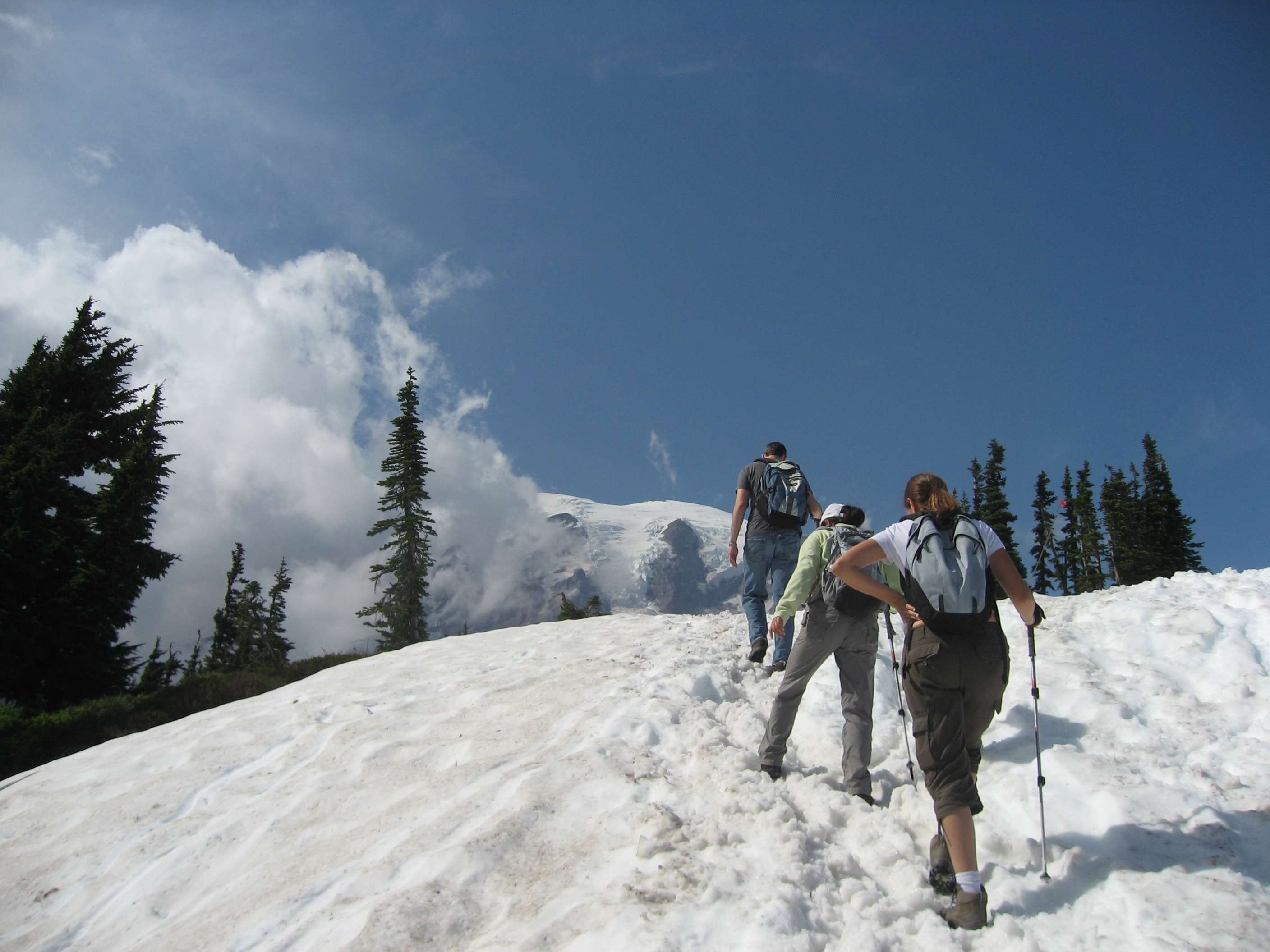
Background image
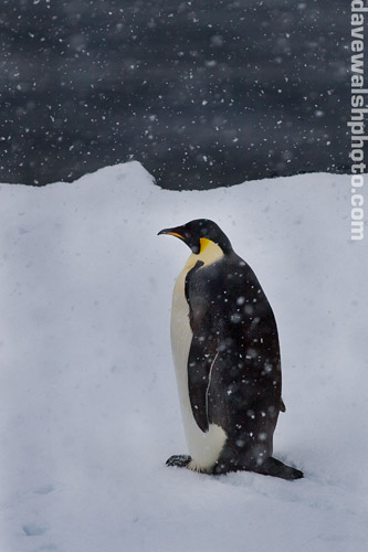
Source image
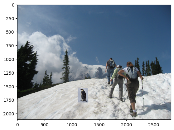
Initial preparation

Poisson blending result
Example 3: Sponge Bob
Background and source images:
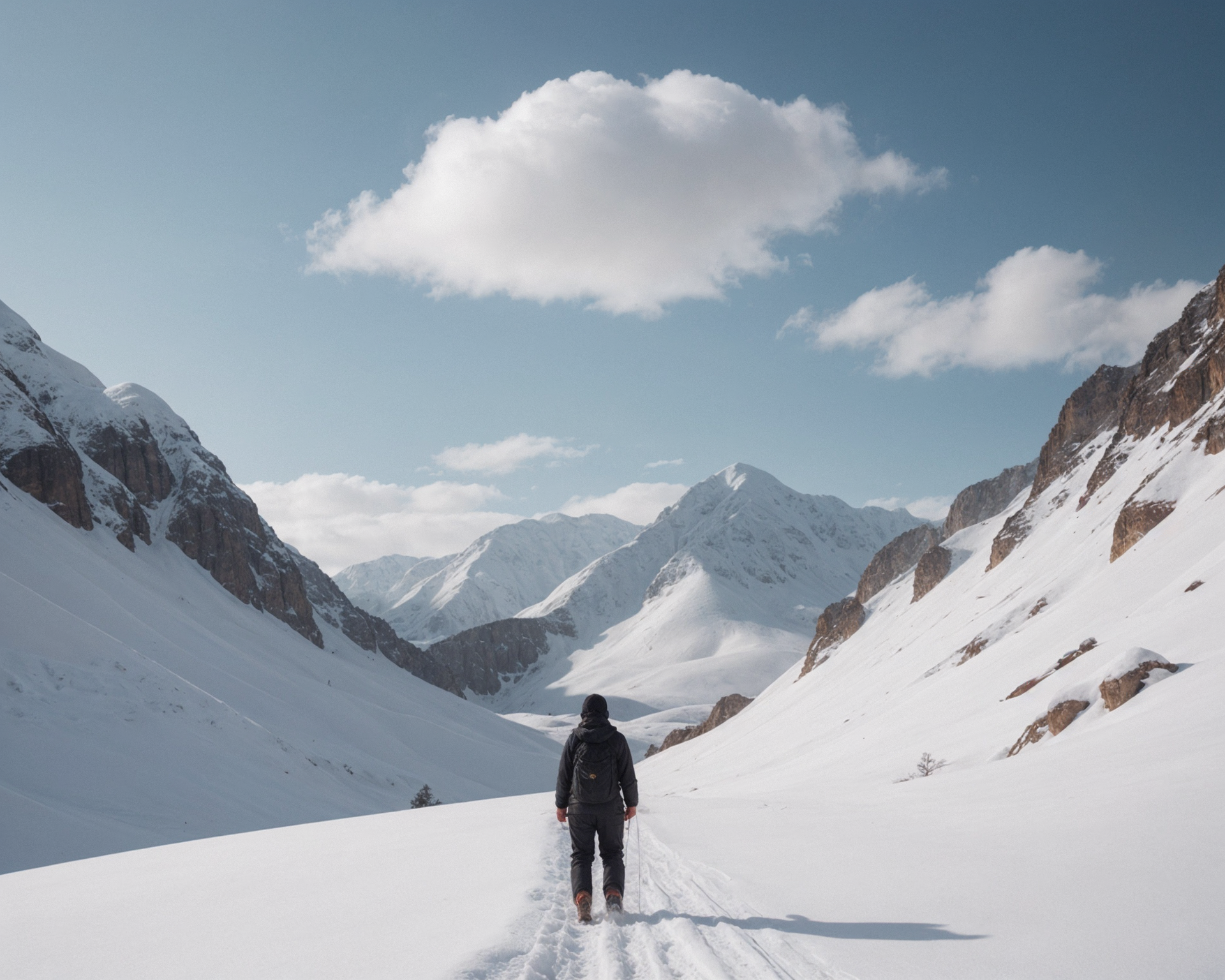
Background image

Source image
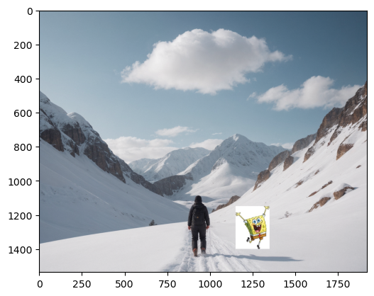
Initial preparation
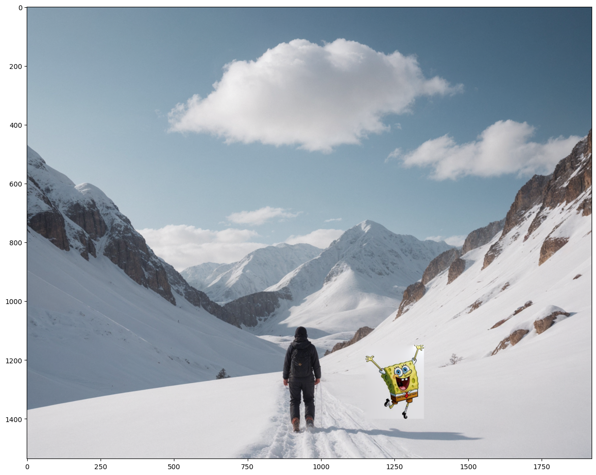
Poisson blending result
Bells & Whistles: Mixed Blending
We also tried adding mixed blending to get a better blending. It is similar to Poisson, but for b, we choose the gradient dependent on the larger one. Formula below: $$ \mathbf{v} = \underset{\mathbf{v}}{\mathrm{argmin}} \left( \sum_{i \in S, j \in N_i \cap S} \left( (v_i - v_j) - d_{ij} \right)^2 + \sum_{i \in S, j \in N_i \cap \neg S} \left( (v_i - t_j) - d_{ij} \right)^2 \right) $$
